What are /r/mathpics' favorite Products & Services?

From 3.5 billion Reddit comments

A consequence of the Prime Number Theorem is that any sequence that's asymptotic to k * N/log(N), for a constant k, will look linear when plotted against the primes.

This is a calculation of energies in a square lattice crystal using the tight binding model. You can see how the function tessellates as its own square lattice. You can play around with the desmos link here:

https://www.desmos.com/calculator/qasm4eyf3j

That is interesting, my implementation was quite a bit more complicated (a recursive approach: calculating the total length, and interpolating each pair of vertices accordingly) I'm astonished you can do this so efficiently, but I do not really get yet how these work. (Do you perhaps know somewhere where this is explained?) Yeah the basic idea is that you can parametrize the curve continuously (which is not true for the inverse). So once I had the parametrization set up, it was only a matter of choosing how many places in what spots. This was basically just a first exercise in order to get into processing, a relatively easy language for visualizing stuff.

EDIT: Oh my god, I just realized who I'm talking to! Just wanted to say that I love your work on Wikipedia!

I've made a simple javascript snippet which generates an SVG you want. Click the "Edit in JS Bin" button at the top-right corner and fill free to adjust parameters. With "Auto-run JS" enabled, it's gonna be dang easy to play with. <http://jsbin.com/lanegigore/4>

EDIT: fixed a bug. relinked to a new revision.

Glad you like it! A goal? hmm.. I was mainly trying to stress test the Paper javascript library. And I've always wanted to see how symplectic integrators compare to the more standard ODE solvers when applied to the n-body problem. I'm not researching these symmetric systems in any way and I have no theoretical analysis for their dynamics.

As far as the instability goes, yes you are right. Over time the numerical error builds up until the symmetry is lost (happens in both videos). The n-body problem is particularly stiff when massive bodies are close together; the gravitational field changes so rapidly that the solver has a hard time integrating over a (seemingly large) fixed timestep. Fortunately, the stiffness is hardly felt by the symmetry, which is why the simulation lasts so long before descending into chaos (~60 realtime seconds for a 2nd order fixed time-step method is pretty impressive imo).

Hey I made that ugly first image!

Always interesting to see these things turn up. Guess you were reading about sine?

Nice fractalization method too.

For a convergent series, you can graph the partial sums and find the asymptote, which is just a horizontal line that they approach. The y-intercept of the line is called the sum of the series.

Now, the series 1 + 2 + 3 + 4 + ⋯ is divergent, but you can do pretty much the same thing! After smoothing out the partial sums, they approach an asymptote which is a parabola, whose y-intercept is the "regularized sum" of the series. The y-intercept is −1/12, as shown in the diagrams.

So to answer your question, it's precisely because the numbers on the stair-step curve are positive that when you extrapolate them back to x=0, you get a negative number. The diagram that shows this most clearly is https://commons.wikimedia.org/wiki/File:Sum1234Asymptote.svg.

The fundamental principle for these graphs is that I've defined a function that takes in a point in mod arg form and outputs another point based on those values. Using the function for a parametric curve yields very pretty results such as this one. To make it even more pleasing to the eye, I've done some fiddling around in The GIMP. Anyway, Enjoy!

https://www.desmos.com/calculator/nlpyswjgbk

Here is a Javascript version you can play with and edit. Use the right/left arrow keys to transition the parameters as in the gif. I'm using the Paper javascript library which is horribly inefficient at rendering pixels (not what it's meant for) -- so it can only do ~2000 iterations z -> F(z) in real time. GLSL would run a lot faster.

Edit: I changed the code so that I'm altering canvas pixel data rather than changing the position of Paper circles. This resulted in a speedup in Safari but a massive slowdown in Chrome for me, so by default it is now only running 100 iterations per frame. The nice thing is that we are no longer using extra memory per iteration and that when the parameters aren't changing, the fractal space will unendingly fill with pixels.

From

https://www.semanticscholar.org/paper/The-Colin-de-Verdi%C3%A8re-graph-parameter-Holst-Lov%C3%A1sz/0049d1d3a8b3226aaa603aca7ab39f3129975e1c/

&nbsp;

Had to repost replacing a previous one because an error was found in the figure. There's this other rather pleasant representation of them, but there is the problem with it that because it has transparency in it the edges don't show-up through reddit rendering! Having somewhat compared them I'm fairly sure they are the same as the ones in the figure posted here.

It's a blasted nuisance that so elementary an item seems to be so difficult to find!

&nbsp;

A linklessly embeddable graph is one that can be constructed in three-dimensional space without any two of its cycles being linked: literally able to be 'drawn' (or constructed) in three-dimensional space such that no cycle passes through any other in the sense of links in a chain 'passing through' each other - ie if they were made of physical substance they could not be separated without breaking it.

For links to the individual graphs:

• cos
• sin

The stationary points don't quite match up with the other graphs, but it's close enough and I'm not sure what the value needed would be.

Unfortunately a cannot be set to infinity, as desmos doesn't support infinity, and don't make a too large, maybe 100-300 is a good maximum before it will probably slow down.

I've heard of it, sounds similar to some of the short stories by Rudy Rucker. Back in my sophomore year ('99), I was given a book called The Fourth Dimension, that introduced me to more of the concepts, after seeing Carl Sagan explain a tesseract in Cosmos.

I did a reverse image search ... Turns out it's from a stock picture on shutterstock
Here's the link:
https://www.shutterstock.com/image-vector/vector-pigeonhole-principle-illustration-flat-icons-373867645?irgwc=1&amp;utm_medium=Affiliate&amp;utm_campaign=Vectors123.com&amp;utm_source=44866&amp;utm_term=

Nice video but I feel like this is missing the justification that the recursive function f(x) = sin(x+sin(x+...) ) actually converges to the fixed point f(x) = sin(x+f(x)). Notice that it's not true for g(x)=tan(x+tan(x+...)), nor h(x)=exp(x+exp(x+...)) even though there are well-defined loci of the fixed points g(x)=tan(x+g(x)) and h(x)=exp(x+h(x)) You can see this for yourself by changing the function in this Desmos graph.

Before you get too excited, this is a graphing error. Zooming in on the plot shows that the discontinuous speckles are actually a closed curve.

https://www.desmos.com/calculator/ngp3ntzqu6

Each 'lobe' is centred at (2*(pi*n-3*pi/4), 2*pi*m ), for integer m, n.

It looks like there are more up-to-date implementations around. This one appears to be Java, not JavaScript, that's the old Sun environment later acquired by Larry Ellison and Oracle.

I expect you could find something modern if you're interested.

https://processing.org/examples/flocking.html

https://github.com/topics/boids-simulation

I'm not sure how I make a makefile for POV-Ray! If you have some steps, I'll do it.

To run the code, you just need to download POV-Ray for free here and then download my .pov file, open it up and hit run.

I made this animation using python with numpy, matplotlib, and animatplot.

The code is on GitHub

To read more on this map see: Chirikov_standard_map.

This animation was made in python with numpy, matplotlib, and animatplot.

Code on GitHub

For more details on the map see: Chirikov_standard_map.

I thought this was cool so I put together an interactive version on Desmos. https://www.desmos.com/calculator/4hlzbiyzru You can change the number of times the smaller circle revolves from 2 to whatever you want.

I see what you're talking about. You are combining the different x-sections together in one image, with movement changing them as one. There is some nice visual continuity in this method. You are right about the rotation version, it will be tricky, since you have to rotate the slice while having the slice itself turn at the same time. I haven't tried that yet.

I actually have a list of functions that plot slices at various 4D depths of T^3, together, including the larger torus surface. It's an idea for an animation. Since I use calcplot at the moment, it requires plotting 9 functions at once, with 8 of them animating.

Plus, I like how you use toratopic notation to communicate! It's very efficient, when speaking of specific slices of specific shapes. Much easier than a giant equation, in my opinion. You know, none of this has been mentioned in a paper, yet, so it's still kind of fringe.

Have you tried to graph all slices of T^3 as one, in desmos? Well, minus the empty intersection ((()z)w). An example is something like this. The rotate functions are the bottom three, all tied in with one rotate parameter per pair of variables.

Just checked, and no, the scaling constant in a square equation won't make trapezoids, but make parallelograms, curiously enough. The triangle equation set up the same way will make diamonds, and arrowheads. Check it out: https://www.desmos.com/calculator/mzi0h9zp8k .

Best way to make sense of it is to look at how a 2D hyperbola comes from a 3D conic: we see the green sheet (in first animation) slicing it off-center, away from the cone tips. The gap between the two hyperbolic curves is just an artifact of being off-center. Moving closer, and the curves will meet, and make an "X" at origin.

In 4D, there are two types of conic surfaces, which make their own type of hyperbola. The surface of a 4D object is a 3D volume, and the surface of a 3D object is a 2D area. Slicing a 2D surface makes 1D line-curves, and slicing a 3D surface makes 2D plane-curves.

The hyperbolas from a 4D conic can be made by revolving one from a 3D conic around different axes, in different directions.

Imagine spinning the hyperbola (from 3D conic) around to make a 2D surface. Around the y-axis will make the 1-sheet, and the x-axis a 2-sheet. The 2-sheet is more identical to a 3D conic hyperbola.

I'm hoping that makes some kind of sense. Packing a ton of numbers together can get confusing, even for me, sometimes!

> What's a good book for 4D geometry?

There's many out there, but I wouldn't know which one is better or worse. I learned it elsewhere.

After looking into it further and reviewing Fourier transforms, I found a more isolated pattern.

Thanks for the tip, I'm gonna keep messing with this.

I guess you could but if you don't understand average end area, and basic cut fill it is not exactly easy to teach through direct message. I would suggest you Google those concepts. There are many books on this very topic https://www.amazon.com/dp/0934041296/ref=cm_sw_r_cp_apa_i_x1YlFbQE1YZYC

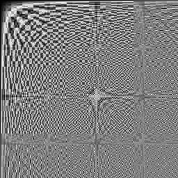
I have an old BASIC program on my calculator that generates a picture that reminds me very much of the images in the article. I think I took it from The Art of Computer Programming but I can't find the page for the life of me.

Does anyone know if it's at all mathematically related to the article? Here's the pseudocode:

For each pixel y,x: If floor(y * y * x * 2^11) % 2 == 1: Turn on pixel y,x